(WIP) Latent Field Discovery in Interacting Dynamical Systems with Neural Fields
We discover global fields in interacting systems, inferring them from the dynamics alone, using neural fields.
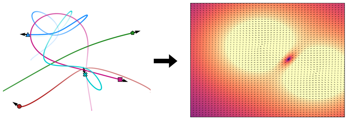 Image credit: Unsplash
TL;DR: Field discovery in interacting systems
We discover global fields in interacting systems, inferring them from the dynamics alone, using neural fields.
Aether, the medium that permeates all throughout space and allows for propagation of light. 💨 🌊 🪨 🔥
Keywords: Graph Neural Networks, Neural Fields, Field Discovery, Equivariance, Interacting Dynamical Systems, Geometric Graphs
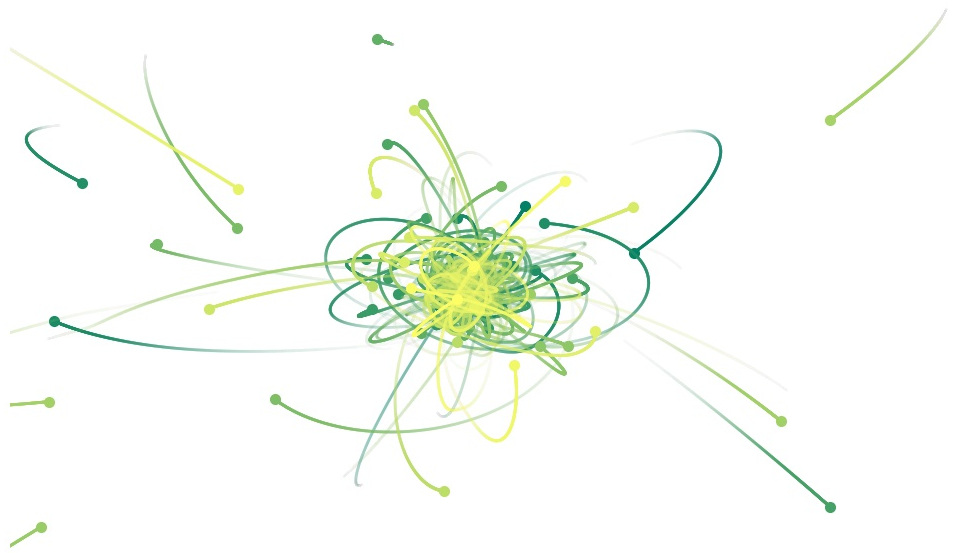
Introduction – Interacting systems are everywhere…
| Colliding particles | N-body systems | Molecules | Traffic scenes |
|---|---|---|---|
Gravitational System
 |
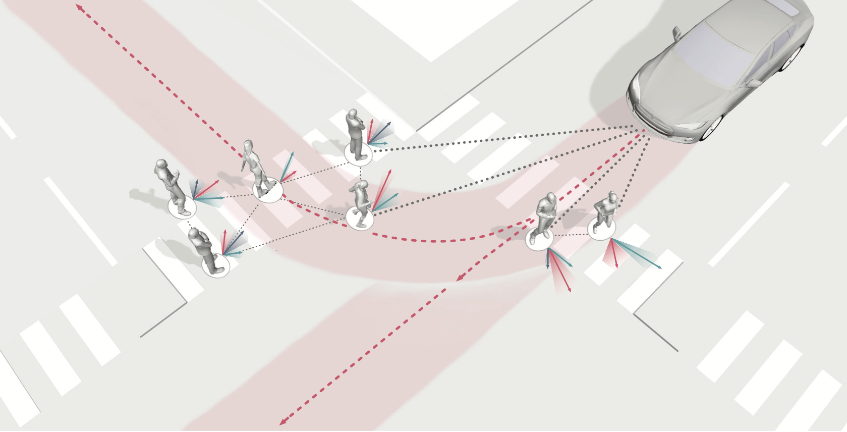
Trajectron Scene
 |
- Colliding particles
- N-body systems
- Molecules
- Traffic scenes
… but they do not evolve in a vacuum
 |
 |
|---|---|
| Figure credit: \cite{eht2019m87} | Figure credit: \cite{nuscenes} |
- Electromagnetic fields
- Gravitational fields
- “Social” fields
- Road network
- Traffic rules
Related work – Equivariant graph networks
Strictly equivariant graph networks exhibit increased robustness and performance, while maintaining parameter efficiency due to weight sharing.
 |
 |
 |
|---|---|---|
| EGNN | LoCS | SEGNN |
However, they are incompatible with global field effects.
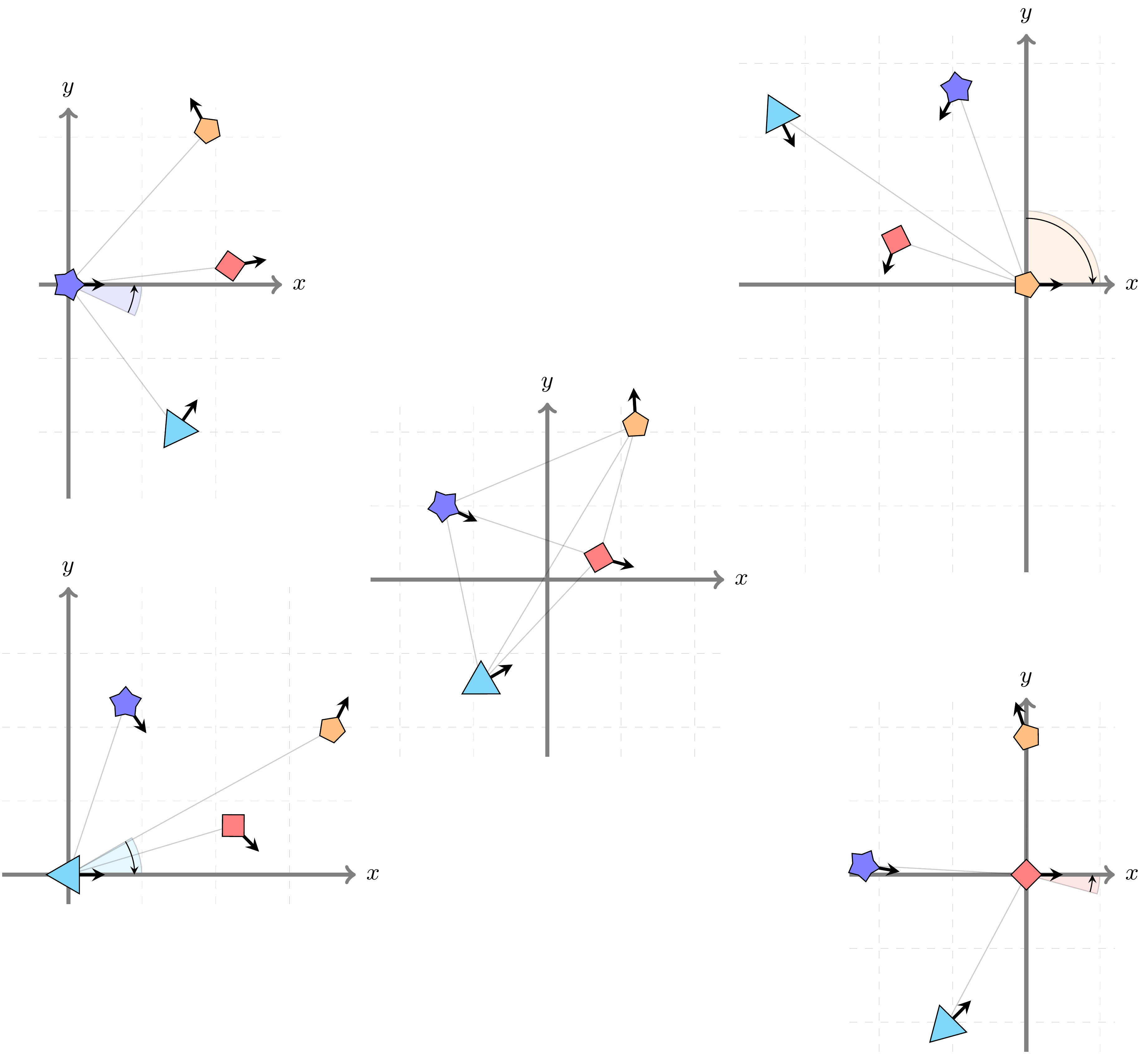
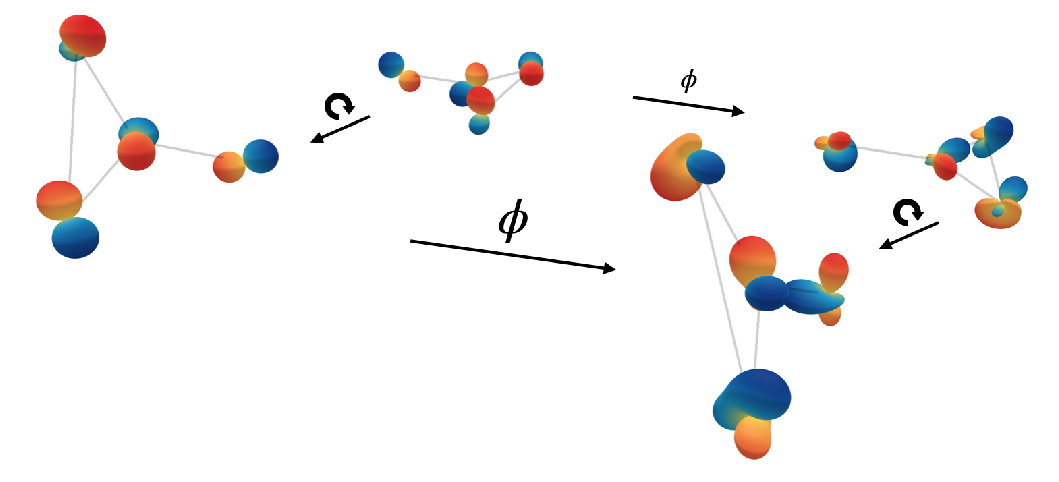
Motivation – Entangled equivariance
Object interactions depend on local information, while underlying field effects depend on global states. Interactions are equivariant to a group of transformations; field effects are not.
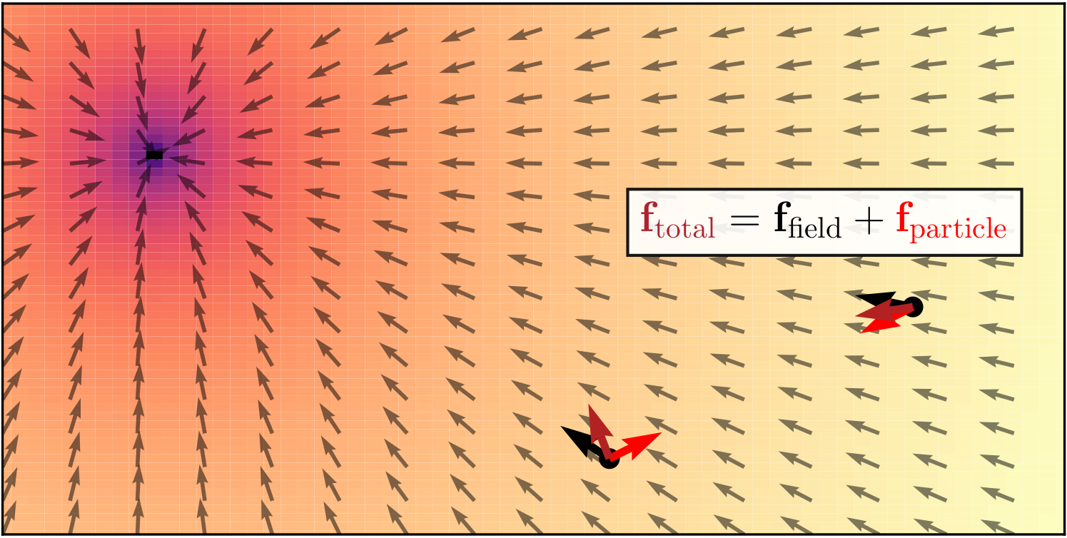
We only observe the net effect of the two constituents. We refer to this as entangled equivariance.
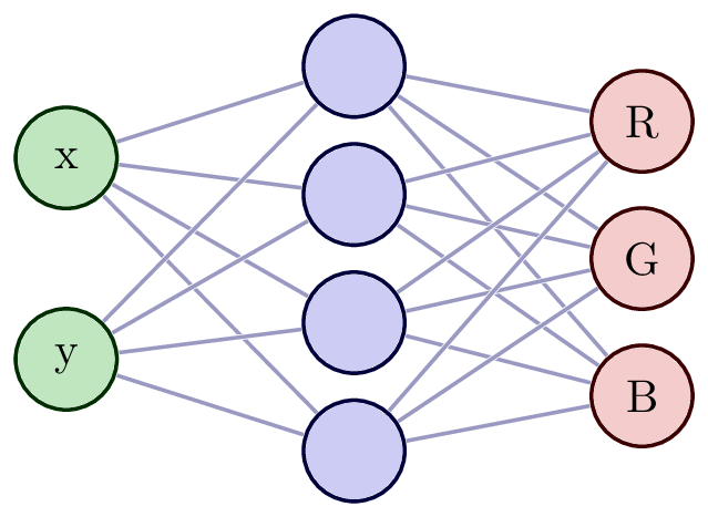
Background – Neural fields primer

-
Grid:
-
MLP:
-
Neural Field:
Background – Equivariant graph network backbone

-
Node Features:
- Positions: $ \mathbf{p}_i $
- Velocities: $ \mathbf{u}_i $
- Orientations: $ \mathbf{\omega}_i $ (for $R\mathbf{v}_i$)
-
Message Passing:
- Local-to-Global Transformation: $ \mathbf{v}{j|i} = \textsc{Global2Local}(\mathbf{v}{j}, \mathbf{v}_{i}) $
- GNN Computation: $ \bm{\Delta}\mathbf{x}{i|i} = \textrm{GNN}(\mathbf{v}{i|i}, {\mathbf{v}{j|i}}{j \in \mathcal{N}(i)}) $
- Local-to-Global Transformation: $ \bm{\Delta}\mathbf{x}i = \textsc{Local2Global}(\bm{\Delta}\mathbf{x}{i|i}) $
-
Node Update: [ \mathbf{\hat{x}}i = \mathbf{x}{i} + \bm{\Delta}\mathbf{x}_i ]
Method – Aether Architecture
We model object interactions with equivariant graph networks [@kofinas2021roto], and field effects with neural fields. We hypothesize that field effects can be attributed to force fields, and therefore, our neural fields learn to discover latent force fields.


The pipeline of our method, Aether. In the latent neural field (Figure 1), a graph aggregation module summarizes the input trajectories in a latent variable $\mathbf{z}$. Query states from input trajectories, alongside $\mathbf{z}$, are fed to a neural field that predicts a latent force field. In the Aether pipeline (Figure 2), a graph network integrates predicted forces with input trajectories to predict future trajectories. The graph aggregation module and the FiLM layers exist only in a dynamic field setting.
Graph Aggregation and Integration Equations:
\begin{columns}
  \begin{column}{0.50\textwidth}
    {\footnotesize
      \begin{align*}
        \mathbf{h}_{j,i}^{(1)} &= f_{e}^{(1)}\left(\left[\mathbf{v}_{j|i}, \highlight{\mathbf{f}_{j|i}}, \mathbf{v}_{i|i}, \highlight{\mathbf{f}_{i|i}}\right]\right) \\
        \mathbf{h}_i^{(1)} &= f_v^{(1)}\left(g_v \left(\left[\mathbf{v}_{i|i}, \highlight{\mathbf{f}_{i|i}}\right]\right) + \frac{1}{|\mathcal{N}(i)|}\smashoperator[r]{\sum_{j \in \mathcal{N}(i)}} \mathbf{h}_{j,i}^{(1)}\right)
      \end{align*}
    }
  </end{column}
  \begin{column}{0.50\textwidth}
    {\footnotesize
      \begin{align*}
        \mathbf{h}_{j,i}^{(l)} &= f_e^{(l)}\left(\left[\mathbf{h}^{(l-1)}_i, \mathbf{h}^{(l-1)}_{j,i}, \mathbf{h}^{(l-1)}_j\right]\right) \\
        \mathbf{h}_{i}^{(l)} &= f_v^{(l)}\left(\mathbf{h}_{i}^{(l-1)} + \frac{1}{|\mathcal{N}(i)|}\smashoperator[r]{\sum_{j \in \mathcal{N}(i)}} \mathbf{h}_{j,i}^{(l)}\right) \\
        \mathbf{\hat{x}}_i &= \mathbf{x}_i + \mathbf{R}_i \cdot f_o\left(\mathbf{h}_i^L\right)
      \end{align*}
    }
  \end{column}
\end{columns}
Visualizations
Miltiadis Kofinas
Postdoctoral researcher, AI for Climate
Graph neural networks, Neural fields, Geometric deep learning